3 List columns
# Libraries
library(tidyverse)
#> ── Attaching packages ─────────────────────────────────────── tidyverse 1.3.1 ──
#> ✓ ggplot2 3.3.5     ✓ purrr   0.3.4
#> ✓ tibble  3.1.4     ✓ dplyr   1.0.7
#> ✓ tidyr   1.1.3     ✓ stringr 1.4.0
#> ✓ readr   2.0.1     ✓ forcats 0.5.1
#> ── Conflicts ────────────────────────────────────────── tidyverse_conflicts() ──
#> x dplyr::filter() masks stats::filter()
#> x dplyr::lag()    masks stats::lag()
library(dcldata)
Recall that tibbles are lists of vectors.
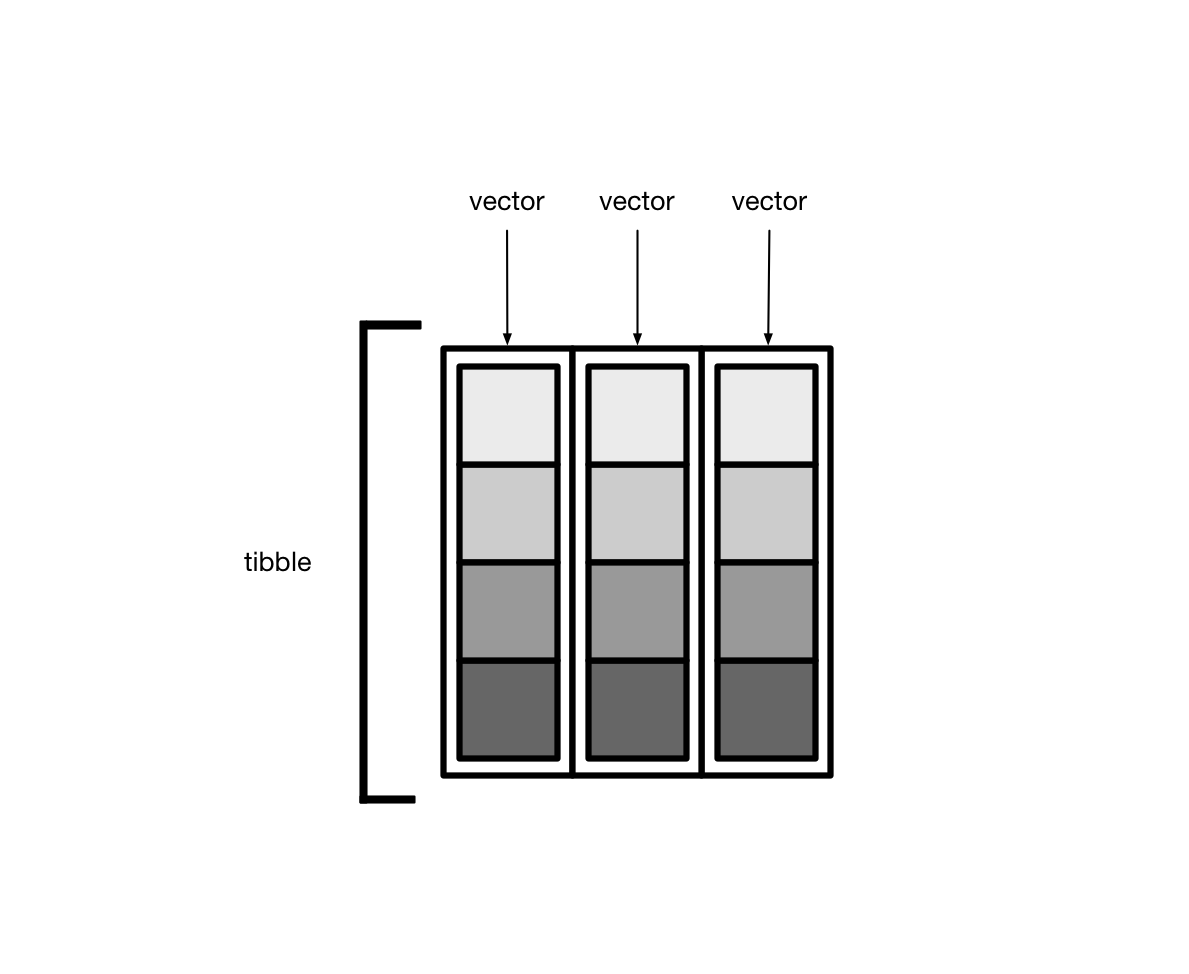
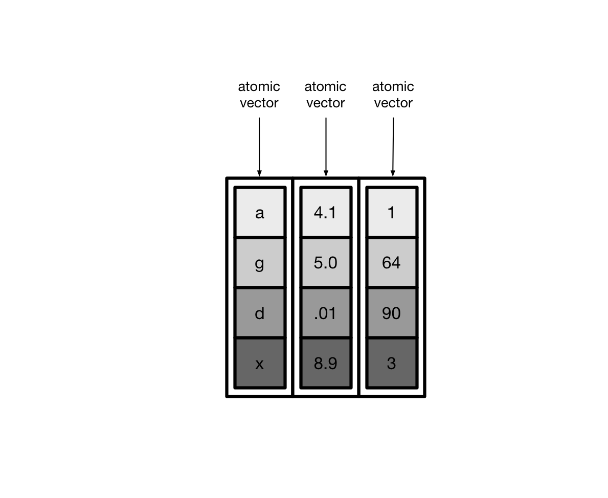
Usually, these vectors are atomic vectors, so the elements in the columns are single values, like “a” or 1.
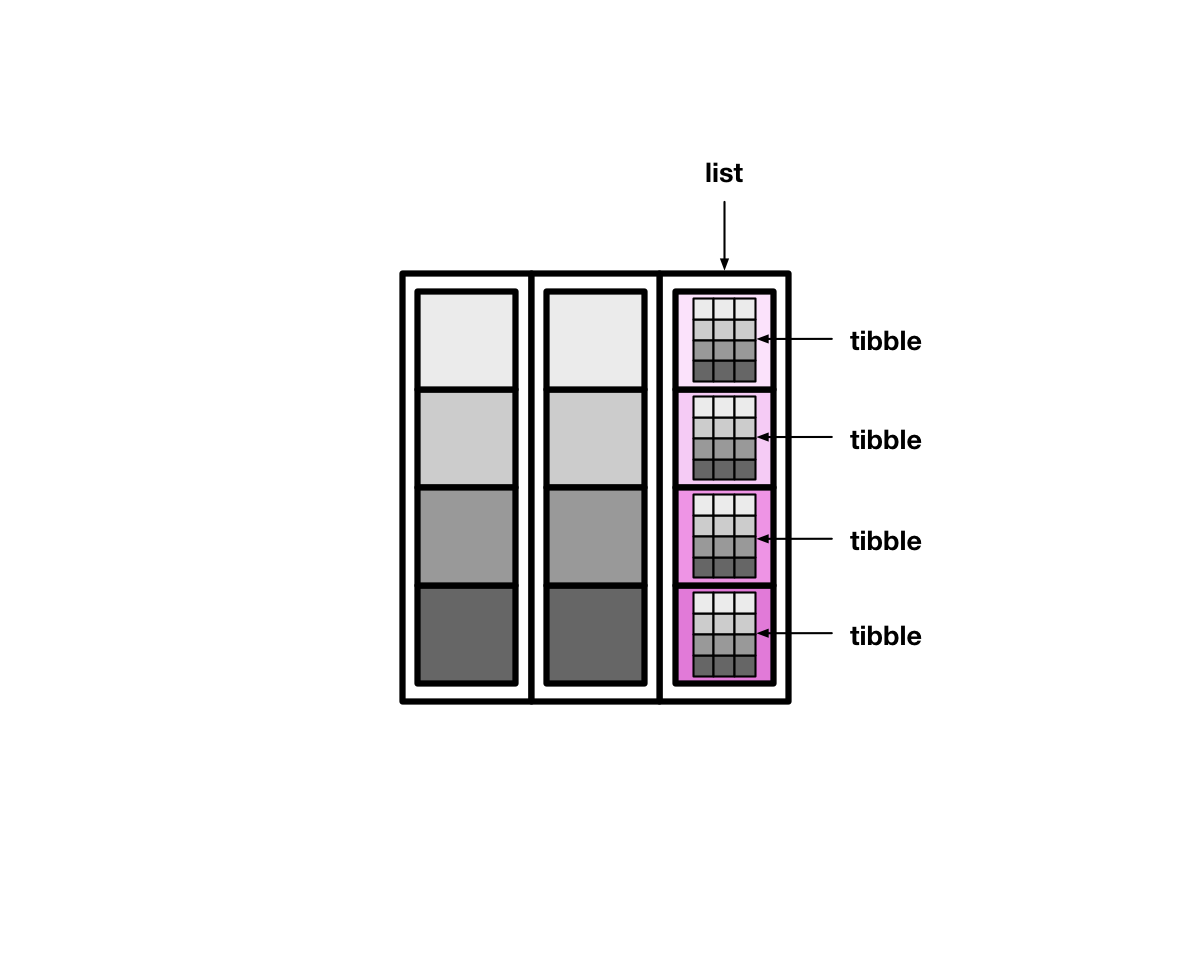
Tibbles can also have columns that are lists. These columns are (appropriately) called list columns.
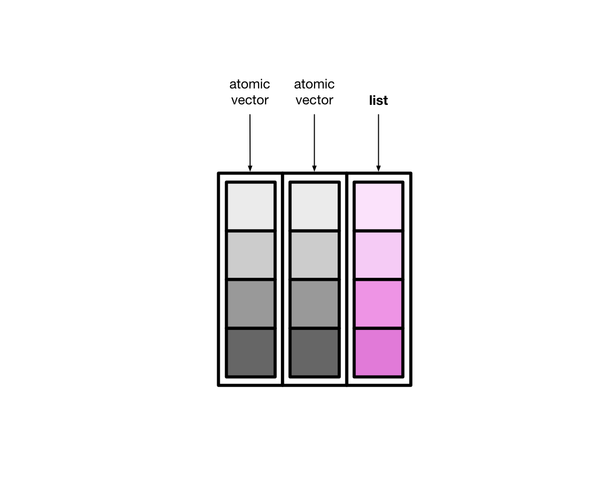
List columns are more flexible than normal, atomic vector columns. Lists can contain anything, so a list column can be made up of atomic vectors, other lists, tibbles, etc.
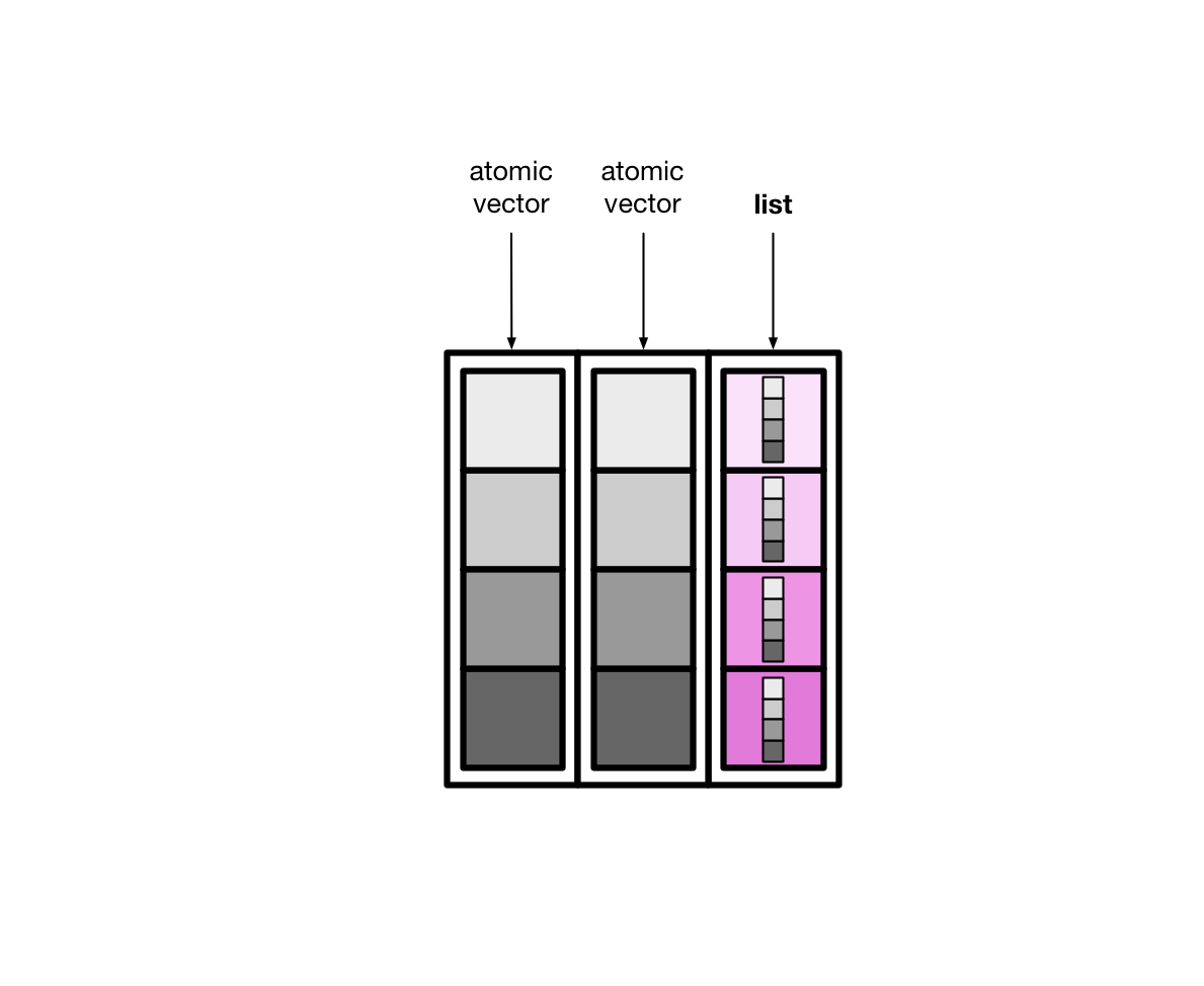
As you’ll see, this can be a useful way to store data. In this chapter, you’ll learn how to create list columns, how to turn list columns back into normal columns, and how to manipulate list columns.
3.1 Creating
Typically, you’ll create list columns by manipulating an existing tibble. There are three primary ways to create list columns:
nest()summarize()andlist()mutate()andmap()
3.1.1 nest()
countries is a simplified version of dcldata::gm_countries, which contains Gapminder data on 197 countries.
countries <-
  gm_countries %>%
  select(name, region_gm4, un_status, un_admission, income_wb_2017)

countries
#> # A tibble: 197 × 5
#>   name                region_gm4 un_status un_admission income_wb_2017
#>   <chr>               <chr>      <chr>     <date>       <chr>
#> 1 Afghanistan         asia       member    1946-11-19   Low income
#> 2 Albania             europe     member    1955-12-14   Upper middle income
#> 3 Algeria             africa     member    1962-10-08   Upper middle income
#> 4 Andorra             europe     member    1993-07-28   High income
#> 5 Angola              africa     member    1976-12-01   Lower middle income
#> 6 Antigua and Barbuda americas   member    1981-11-11   High income
#> # … with 191 more rows
The tidyr function nest() creates list columns of tibbles.
Pass nest() the names of the columns to put into each individual tibble. nest() will create one row for each unique value of the remaining variables. For example, say we select just two columns from countries
countries %>%
  select(region_gm4, name)
#> # A tibble: 197 × 2
#>   region_gm4 name
#>   <chr>      <chr>
#> 1 asia       Afghanistan
#> 2 europe     Albania
#> 3 africa     Algeria
#> 4 europe     Andorra
#> 5 africa     Angola
#> 6 americas   Antigua and Barbuda
#> # … with 191 more rows
and then nest name.
regions <-
  countries %>%
  select(region_gm4, name) %>%
  nest(countries = name)

regions
#> # A tibble: 4 × 2
#>   region_gm4 countries
#>   <chr>      <list>
#> 1 asia       <tibble [59 × 1]>
#> 2 europe     <tibble [49 × 1]>
#> 3 africa     <tibble [54 × 1]>
#> 4 americas   <tibble [35 × 1]>
nest() created one tibble for each region_gm4.
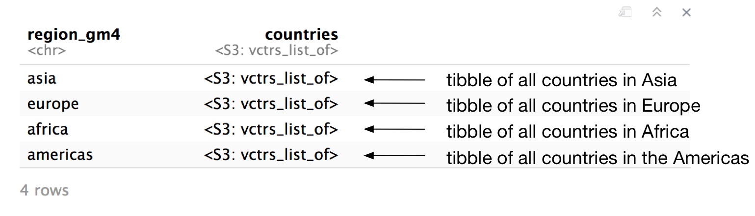
Each of these tibbles contains all the countries that belong to the continent.
regions$countries[[1]]
#> # A tibble: 59 × 1
#>   name
#>   <chr>
#> 1 Afghanistan
#> 2 Australia
#> 3 Bahrain
#> 4 Bangladesh
#> 5 Bhutan
#> 6 Brunei
#> # … with 53 more rows
The entire column is a list.
typeof(regions$countries)
#> [1] "list"
If we nest multiple variables, the individual tibbles will have multiple columns.
regions_data <-
  countries %>%
  nest(data = c(name, un_status, un_admission, income_wb_2017))

regions_data
#> # A tibble: 4 × 2
#>   region_gm4 data
#>   <chr>      <list>
#> 1 asia       <tibble [59 × 4]>
#> 2 europe     <tibble [49 × 4]>
#> 3 africa     <tibble [54 × 4]>
#> 4 americas <tibble [35 × 4]>regions_data$data[[1]]
#> # A tibble: 59 × 4
#> name un_status un_admission income_wb_2017
#> <chr> <chr> <date> <chr>
#> 1 Afghanistan member 1946-11-19 Low income
#> 2 Australia member 1945-11-01 High income
#> 3 Bahrain member 1971-09-21 High income
#> 4 Bangladesh member 1974-09-17 Lower middle income
#> 5 Bhutan member 1971-09-21 Lower middle income
#> 6 Brunei member 1984-09-21 High income
#> # … with 53 more rowsYou can specify columns to nest using the same syntax as select().
countries %>%
  nest(data = !region_gm4)
#> # A tibble: 4 × 2
#>   region_gm4 data
#>   <chr>      <list>
#> 1 asia       <tibble [59 × 4]>
#> 2 europe     <tibble [49 × 4]>
#> 3 africa     <tibble [54 × 4]>
#> 4 americas   <tibble [35 × 4]>
You can also create multiple list columns at once.
countries %>%
  nest(countries = name, data = c(name, contains("un"), income_wb_2017))
#> # A tibble: 4 × 3
#>   region_gm4 countries         data
#>   <chr>      <list>            <list>
#> 1 asia       <tibble [59 × 1]> <tibble [59 × 4]>
#> 2 europe     <tibble [49 × 1]> <tibble [49 × 4]>
#> 3 africa     <tibble [54 × 1]> <tibble [54 × 4]>
#> 4 americas   <tibble [35 × 1]> <tibble [35 × 4]>
3.1.2 summarize() and list()
You’ve used group_by() and summarize() to collapse groups into single rows. We can also use summarize() to create a list column, where each element is a vector, list, or tibble.
If you supply list() with multiple atomic vectors, it will create a list of atomic vectors.
list(c(1, 2, 3), c("a", "b", "c"))
#> [[1]]
#> [1] 1 2 3
#>
#> [[2]]
#> [1] "a" "b" "c"
We can use summarize() and list() to create a list of atomic vectors where each vector corresponds to one region_gm4. For example, the following creates a list column of countries.
countries_collapsed <-
  countries %>%
  group_by(region_gm4) %>%
  summarize(countries = list(name))

countries_collapsed
#> # A tibble: 4 × 2
#>   region_gm4 countries
#>   <chr>      <list>
#> 1 africa     <chr [54]>
#> 2 americas   <chr [35]>
#> 3 asia       <chr [59]>
#> 4 europe     <chr [49]>
The countries column is similar to the one created earlier with nest(), except each element is an atomic vector, not a tibble.
typeof(countries_collapsed$countries[[1]])
#> [1] "character"
What if we want to manipulate each vector before creating the list column? For example, say we want to arrange all country names alphabetically. The following doesn’t work:
countries %>%
  group_by(region_gm4) %>%
  summarize(countries = sort(name))
#> # A tibble: 197 × 2
#> # Groups:   region_gm4 [4]
#>   region_gm4 countries
#>   <chr>      <chr>
#> 1 africa     Algeria
#> 2 africa     Angola
#> 3 africa     Benin
#> 4 africa     Botswana
#> 5 africa     Burkina Faso
#> 6 africa     Burundi
#> # … with 191 more rows
You need to collect all the atomic vectors into a list.
countries %>%
  group_by(region_gm4) %>%
  summarize(countries = list(sort(name)))
#> # A tibble: 4 × 2
#>   region_gm4 countries
#>   <chr>      <list>
#> 1 africa     <chr [54]>
#> 2 americas   <chr [35]>
#> 3 asia       <chr [59]>
#> 4 europe     <chr [49]>
Here’s another example, which only stores in countries only the countries that begin with “A”.
a_countries <-
  countries %>%
  group_by(region_gm4) %>%
  summarize(countries = list(str_subset(name, "^A")))

a_countries
#> # A tibble: 4 × 2
#>   region_gm4 countries
#>   <chr>      <list>
#> 1 africa     <chr [2]>
#> 2 americas   <chr [2]>
#> 3 asia       <chr [2]>
#> 4 europe     <chr [5]>

a_countries$countries[[1]]
#> [1] "Algeria" "Angola"
3.1.3 mutate()
The third way to create a list column is use to rowwise() and mutate(). For example, the following creates a list column where the element for each country is a vector of random numbers.
countries %>%
  select(name) %>%
  rowwise() %>%
  mutate(random = list(rnorm(n = str_length(name)))) %>%
  ungroup()
#> # A tibble: 197 × 2
#>   name                random
#>   <chr>               <list>
#> 1 Afghanistan         <dbl [11]>
#> 2 Albania             <dbl [7]>
#> 3 Algeria             <dbl [7]>
#> 4 Andorra             <dbl [7]>
#> 5 Angola              <dbl [6]>
#> 6 Antigua and Barbuda <dbl [19]>
#> # … with 191 more rows
3.2 Unnesting
To transform a list column into normal columns, use unnest(). Here’s our tibble with a list column of country names.
regions
#> # A tibble: 4 × 2
#>   region_gm4 countries
#>   <chr>      <list>
#> 1 asia       <tibble [59 × 1]>
#> 2 europe     <tibble [49 × 1]>
#> 3 africa     <tibble [54 × 1]>
#> 4 americas   <tibble [35 × 1]>
Supply the cols argument of unnest() with the name of the columns to unnest.
regions %>%
  unnest(cols = countries)
#> # A tibble: 197 × 2
#>   region_gm4 name
#>   <chr>      <chr>
#> 1 asia       Afghanistan
#> 2 asia       Australia
#> 3 asia       Bahrain
#> 4 asia       Bangladesh
#> 5 asia       Bhutan
#> 6 asia       Brunei
#> # … with 191 more rows
3.3 Manipulating
To manipulate list columns, you’ll often find it helpful to use row-wise operations. For example, say we want to find the number of countries in each continent. Here’s regions again.
regions
#> # A tibble: 4 × 2
#>   region_gm4 countries
#>   <chr>      <list>
#> 1 asia       <tibble [59 × 1]>
#> 2 europe     <tibble [49 × 1]>
#> 3 africa     <tibble [54 × 1]>
#> 4 americas   <tibble [35 × 1]>
We can’t call length() directly on countries, because we’ll just get the length of the entire column.
regions %>%
  mutate(num_countries = length(countries))
#> # A tibble: 4 × 3
#>   region_gm4 countries         num_countries
#>   <chr>      <list>                    <int>
#> 1 asia       <tibble [59 × 1]>             4
#> 2 europe     <tibble [49 × 1]>             4
#> 3 africa     <tibble [54 × 1]>             4
#> 4 americas   <tibble [35 × 1]>             4
Instead, we need to iterate over each element or row of countries separately.
regions %>%
  rowwise() %>%
  mutate(num_countries = nrow(countries)) %>%
  ungroup()
#> # A tibble: 4 × 3
#>   region_gm4 countries         num_countries
#>   <chr>      <list>                    <int>
#> 1 asia       <tibble [59 × 1]>            59
#> 2 europe     <tibble [49 × 1]>            49
#> 3 africa     <tibble [54 × 1]>            54
#> 4 americas   <tibble [35 × 1]>            35
Note that we need to use nrow() because each element of countries is actually a tibble.
This code finds the proportion of a region’s country names that end in “a”.
regions %>%
  rowwise() %>%
  mutate(
    ends_in_a = sum(str_detect(countries$name, "a$")) / nrow(countries)
  ) %>%
  ungroup() %>%
  arrange(desc(ends_in_a))
#> # A tibble: 4 × 3
#>   region_gm4 countries         ends_in_a
#>   <chr>      <list>                <dbl>
#> 1 americas   <tibble [35 × 1]>     0.457
#> 2 africa     <tibble [54 × 1]>     0.407
#> 3 europe     <tibble [49 × 1]>     0.347
#> 4 asia       <tibble [59 × 1]>     0.271